Introduction
2024 saw the first 100m$+ training runs, while the insane compute requirements of training Large Language Models is no secret, this jump brought more attention to the need to find tricks and methods to optimize both the transformers architecture and the training process (infrastructure).
The biggest / most successful of these optimizations in recent times has been flash attention (cite here), an idea that focuses on how the compute hungry (O(N)^2) self attention mechanism is computed, by moving attention matrices to SRAM. (Essentially the idea here is that we tried to optimize self attention by modifying how the operation is performed on the GPU.). The trend of squeezing out performance as much as possible from the training infrastructure continued, with researchers writing their own optimal cuda kernels. Deepseek took this a step further, writing their own distributed file system (Fire Flyer FileSystem), a new attention mechanism (MultiHead Latent Attention with custom kernels), a highly tuned communication library for mixture-of-experts models (Deep-EP), and Deep Gemm, an FP-8 optimized matrix multiplication kernel library.
However, looking beyond the model itself, the cross entropy loss function has had a memory problem that has quietly crept up with a recent trend in LLM development, Large Vocabulary sizes.
A bit on Cross Entropy
Cross Entropy originates from information theory, and is a function that measures the difference between two probability distributions. In Machine Learning, the Cross Entropy Loss function is used in calculating the loss between the model’s predicted probabilities and the dataset’s true value.
LLM Training
Large language models are trained by autoregressively predicting the next token in a corpus, this corpus could vary from the entire internet, scientific texts and literature, textbooks etc in large scale pretraining, to smaller datasets on specific niches or domains(as in finetuning).
Given a sequence with N-1 tokens, a large language model can be defined as :
\[ P(x) = \prod_{i=1}^{N} P(x_i | x_1 \ldots x_{i-1}) \]Thus, we could say a large language model parameterizes a probability distribution over all possible tokens in it’s vocabulary. this probability distribution is used to decide the next token in the sequence.
This probability distribution is encoded in the model’s weights (Transformer Architecture), consisting of a backbone network (transformer layers) and a final classifier output layer (a simple neural network with an intermediate layer). (Image of the GPT Architecture)
The output of the backbone network is popularly referred to as an embedding vector. These embeddings are the model’s representation of a token, generated by multiple self-attention layers where the model encodes contextual information into each token’s embeddings.
\[ E = f(x1 . . . xi−1) \]where
\[ f(x_1 \ldots x_{i-1}) \]signifies the backbone network (Transformer layers)
These embeddings are then fed as inputs to the classifier layer C⊤ to produce unnormalized Log Probabilities (Logits)
\[ logits = C^\top f(x_1 \ldots x_{i-1}) \]These logits are then converted to a probability distribution over all the tokens in the model’s vocabulary (V), using the softmax activation function and taken as the model’s prediction for the next token.
\[ \text{softmax}_k(\mathbf{v}) = \frac{\exp(v_k)}{\sum_j \exp(v_j)} \]where vk = Logits for the desired class
vj = Logits for all indices j in the model’s Vocabulary (V)
The output of the softmax activation function is our desired probability distribution, and is used in generating the next token in inference or calculating the loss score during training.
Thus we could summarize a language model as:
\[ P(x_i | x_1 \ldots x_{i-1}) = \text{softmax}_{x_i}(C^\top f(x_1 \ldots x_{i-1})) \]Like with every other classification problem in machine learning, we take the class with the highest predicted probability as the model’s prediction, in our case, the model’s predicted next token in the sequence, which could be anything from a simple “.” to the answer to the question of God, the Universe and life.
This process is autoregressive, with the predicted token appended to the model’s next input sequence to predict the next token, and so on, looping through the entire training corpus.
Training a Language model, is like training any other deep learning based classifier in this sense, the model makes a prediction (next word), a loss (Cross Entropy) is computed by using the model’s predicted probabilities and the true value(the actual next token in the sequence), this loss is used to compute gradients that are backpropagated through the model to adjust it’s weight, repeatedly till a desired loss value is achieved or a desired number of training tokens are exhausted.
During training, the langauge model aims to minimize the cross entropy loss or maximize the probability of predicting the right token
\[ \ell(\hat{x}) = \sum_{i=1}^{N} \log P(\hat{x}_i|\hat{x}_1, \ldots, \hat{x}_{i-1}) \]Given a training batch with batch size 8, containing sequences of length 2048 (GPT 5.2 is rumoured to have around 400k),
we have our input tensor x with shape: [8, 2048].
Thus our model takes 8 sequence with 2048 tokens each as input.
After a forward pass through the model, the backbone network (transformer layers) generates an embedding matrix E of shape:
\[ B, S, D \]where B = Batch Size (8), S = Sequence Length (2048) D = Hidden Dimension
D represents the size of our embedding vectors. Essentially every token in the batch gets an embedding vector computed.
Note: E is computed in parrallel for all tokens, thanks to teacher forcing, the parallel nature of the transformer layers (self-attention) and broadcasting in modern deep learning frameworks like PyTorch.
These embeddings are then passed through the Classifier C⊤, to generate the logits. These logits are of shape:
\[ B, S, V \]where V = Vocabulary Size
Thus for every token, we predict the log probabilities for every token in the model’s vocab. This is also done in parrallel.
As mentioned earlier, the Logits are then used to generate the probability distribution, used in computing the cross entropy loss.
The Memory Problem
At inference, sampling from the model’s predicted probabilities is efficient for any token as it is independent of the sequence length, since the model produces one token at a time at each step using the hidden state E of the last token in the sequence.
During Training, for a sequence
\[ (x1, . . . , xN) \]the model’s outputs
\[ f(x1), f(x1, x2), . . . , f(x1, . . . , xN) \]are also computed in parallel. However, extra memory is required for saving the activation outputs of each layer and optimizer states for computing the gradients for the backward pass, together with the model’s weight.
Researchers over the years have come up with different optimization techniques like activation checkpointing, Gradient Accumulation etc, to help optimize memory consumption during training.
However, despite optimizing the memory consumption of gradients, activations and optimizer states, the unsuspecting final layer (computing the cross entropy loss) occupies most of the model’s memory footprint at training time.
The Cut Cross Entropy team at Apple, noted in their paper that for Large Vocabulary models (See why Large Vocabularies are better), the log probabilites materialized for computing the cross entropy accounts for 40% to 90% (smaller models with larger vocabularies) of the memory consumption at training. With LLMs, larger vocabularies mean better text compression, and subsequently less compute during inference, the models also have a implicit representation for more tokens.
To Understand why the cross entropy layer hogs so much memory during training, let’s look closely at how the cross entropy loss is computed.
The cross entropy loss is given as:
\[ \ell_i(x) = \log \text{softmax}_{x_i}(C^\top E_i) \]C⊤ and E maintain their values as the Classifier and Embedding matrices.
we know the softmax function to be:
\[ \frac{\exp(C^\top_{x_i} E_i)}{\sum_j \exp(C^\top_j E_i)} \]thus, the cross entropy loss can be written as:
\[ \ell_i(x) = \log \frac{\exp(C^\top_{x_i} E_i)}{\sum_j \exp(C^\top_j E_i)} \]taking the log of the numerator and denominator gives:
\[ \ell_i(x)= \log \exp(C^\top_{x_i} E_i) - \log \sum_j \exp(C^\top_j E_i) \]which finally reduces to
\[ \ell_i(x) = C^\top_{x_i} E_i - \log \sum_j \exp(C^\top_j E_i) \]Using Gemma 2(8b), with a vocabulary size of 250,000 as an example:
To compute the cross entropy loss,
we must first perform an indexed matrix multplicaton
\[ C^\top_{x_i} E_i \]This is a simple dot product between the column vector $C^\top_{x_i}$which corresponds to the classifier weights for the target class $x_i$ and the Embedding vector $E_I$
To compute the second part of the equation, the Log Sum Exp, we must first compute a bunch of intermediary tensors. To compute the Log Sum Exp,
\[ \log \sum_j \exp(C^\top_j E_i) \]we first compute
the logits for all tokens in the vocab
\[(C^\top_j E_i) \]Find the max of the computed logits
Substract the logits from the max (This is done for numerical stability to prevent floating point underflows)
Compute the exponent of the normalized logits
\[exp(C^\top_j E_i)\]sum the exponents
\[\sum_j \exp(C^\top_j E_i)\]finally, we take the log of the sums and store it as the loss.
Each of these steps requires intermediary tensors of size $ B, S, V$ in global memory.
Gemma2 has a max sequence length of 80,000 and a vocab size of 256,128 assuming a batch size of 8 and Bf16 floating points precision;
The total memory requirement sums to
\[ 8*800000*256128*2 = 256gb \]about 256gb of memory, just to store the intermediate tensors required to compute the cross entropy loss, accounting for over 90% of the total memory consumption of the training process.
Cut Cross Entropy
Cut Cross Entropy approaches the memory problem through efficient forward and backward passes using custom fused kernels.
Forward Pass
The cross entropy loss is once again given as:
\[ \ell_i(x) = C^\top_{x_i} E_i - \log \sum_j \exp(C^\top_j E_i) \]We can break this into two separate steps , the indexed matrix multiplication and the Log Sum Exp.
As mentioned earlier, a naive computation of the indexed matrix multiplication involves either indexing the classifier weight matrix (CI) with a memory cost of O(ND) in the worst case scenario, and then performing the dot product, or computing
\[(C^\top_j E_i) \]which materializes the logits for every token and then indexing into the result to get the logit for the target class, with an O(N|V |) memory cost.
Cut Cross Entropy uses a different approach,
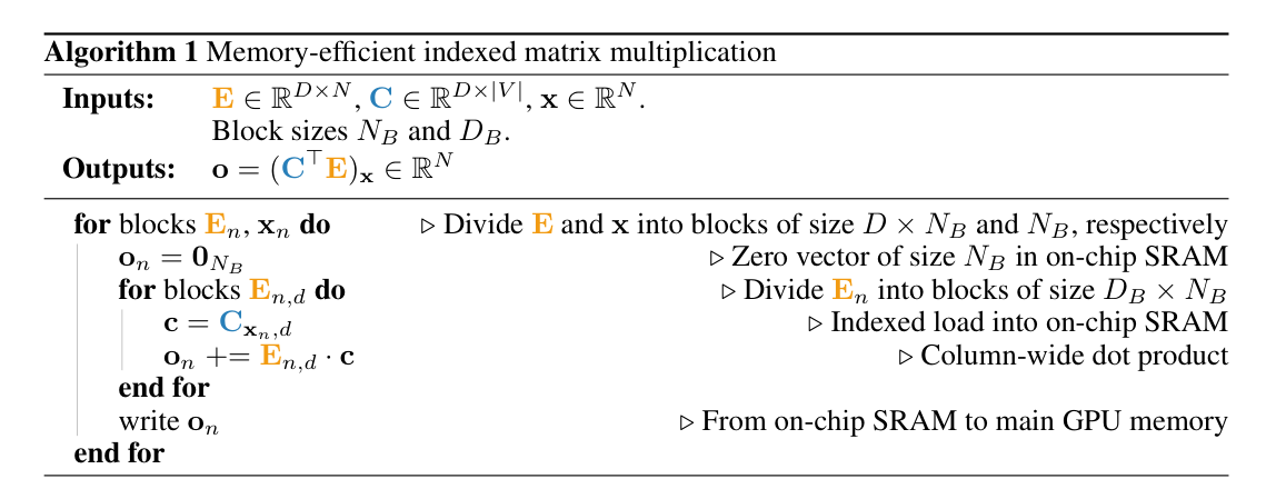
The above algorithm, uses tiling to efficiently materialize blocks of E and C in the on-chip SRAM (shared memory) on the GPU. Rather than materializing all the logits in global memory, we accumulate the dot product on each tile in o, then write final dot product to global memory for a block,
?? to include values on how much memory is saved using tiling.
This implementation is efficient and fast, because we can now compute the dot product C E without storing large tensors in memory.
The triton implementation for this is shown below
import triton
import triton.language as tl


def _indexed_neg_dot_forward_kernel(
    E,
    C,
    Inds,
    Valids,
    Out,
    B,
    D,
    stride_eb,
    stride_ed,
    stride_cv,
    stride_cd,
    stride_ib,
    stride_vb,
    B_BIN,
    BLOCK_B: tl.constexpr,
    BLOCK_D: tl.constexpr,
    GROUP_B: tl.constexpr,
    HAS_VALIDS: tl.constexpr,
    EVEN_D: tl.constexpr,
    SHIFT: tl.constexpr,
):
    pid = tl.program_id(axis=0)
    num_b_chunks = tl.cdiv(B, BLOCK_B)
    num_d_chunks = tl.cdiv(D, BLOCK_D)
    num_d_in_group = GROUP_B * num_d_chunks
    group_id = pid // num_d_in_group
    first_pid_b = group_id * GROUP_B
    group_size_b = min(num_b_chunks - first_pid_b, GROUP_B)
    pid_b = first_pid_b + ((pid % num_d_in_group) % group_size_b)
    pid_d = (pid % num_d_in_group) // group_size_b

    offs_b = (tl.arange(0, BLOCK_B) + pid_b * BLOCK_B) % B
    if HAS_VALIDS:
        offs_b = tl.load(Valids + stride_vb * offs_b)

    offs_d = tl.arange(0, BLOCK_D) + pid_d * BLOCK_D
    e_ptrs = E + (stride_eb * offs_b[:, None] + stride_ed * offs_d[None, :])
    if EVEN_D:
        e = tl.load(e_ptrs)
    else:
        e = tl.load(e_ptrs, mask=offs_d[None, :] < D, other=0.0)

    inds = tl.load(Inds + stride_ib * ((offs_b + 1) if SHIFT else offs_b))

    c_ptrs = C + (inds[:, None] * stride_cv + offs_d[None, :] * stride_cd)
    if EVEN_D:
        c = tl.load(c_ptrs)
    else:
        c = tl.load(c_ptrs, mask=offs_d[None, :] < D, other=0.0)

    offs_b = tl.arange(0, BLOCK_B) + pid_b * BLOCK_B
    out_ptrs = Out + offs_b
    dot = (e * c).to(tl.float32)
    neg_dot = -tl.sum(dot, 1).to(out_ptrs.dtype.element_ty)
    tl.atomic_add(out_ptrs, neg_dot, mask=offs_b < B)
The second part of our equation, the Log Sum Exp, is also implemented using a