Introduction

Whilst working on pretraining SabiYarn in 2025, I came across a really interesting paper by a team at Apple called “Cut Your Losses In Large-Vocabulary Language Models”, they had a very interesting proposition - the cross entropy loss function has had a memory problem that has quietly crept up with a recent trend in LLM development, Large Vocabulary sizes. The paper introduces an optimised kernel for computing the cross entropy, called Cut Cross Entropy. Taking the Gemma 2 (2B) model as an example, CCE reduces the memory footprint of the cross entropy loss computation during training from 24 GB to 1 MB, and the total training-time memory consumption of the classifier head from 28 GB to 1 GB.

Deepseek’s emergence in December 2024 marked a significant turning point in the LLM industry. As major AI labs continued to scale model performance through ever-increasing compute budgets, DeepSeek showed that gains in performance, cost and scalability came from optimizing the whole stack, from compute kernels to optimized memory access, networking and storage.While pretraining DeepSeek V3, the team developed an open source distributed file system 3FS (Fire-Flyer- FileSystem) optimized for high throughput training, a new attention mechanism (MultiHead Latent Attention with custom kernels), a highly tuned communication library for mixture-of-experts models (Deep-EP), and Deep GEMM, an FP-8 optimized matrix multiplication kernel library.

A bit on Cross Entropy

Cross Entropy originates from information theory, and is a function that measures the difference between two probability distributions. In machine learning, the Cross Entropy loss function is used in calculating the loss between a model’s predicted probabilities and the dataset’s true value.

LLM Pretraining

Large language models are trained by autoregressively predicting the next token in a dataset, this dataset could vary from the entire internet, scientific texts and literature, textbooks etc in large scale pretraining, to smaller datasets on specific niches or domains as in model fine-tuning.

Given a sequence with N-1 tokens, a large language model can be defined as :

\[ P(x) = \prod_{i=1}^{N} P(x_i | x_1 \ldots x_{i-1}) \]

That is, a large language model parameterizes a probability distribution over all possible tokens in it’s vocabulary. This probability distribution is used to predict the next token in a sequence.

The probability distribution is encoded as weights in the model’s architecture, consisting of a backbone network (transformer layers) and a final classifier layer.

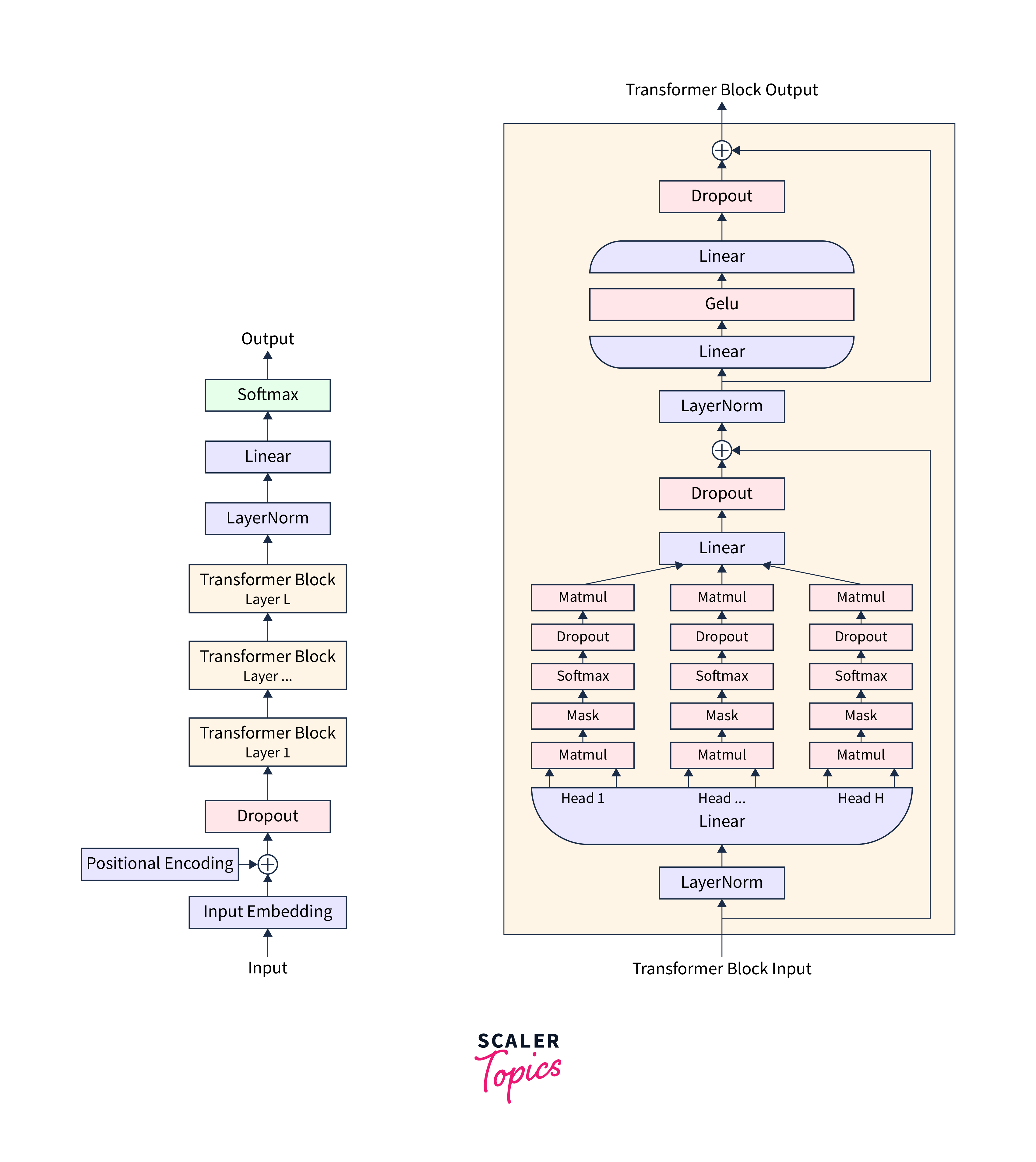
The output of the backbone network is often referred to as an embedding vector. These embeddings are the model’s representation of a token, generated by multiple self-attention layers where the model encodes contextual information from the sequence into each token’s embeddings.

\[ E = f(x1 . . . xi−1) \]

where

\[ f(x_1 \ldots x_{i-1}) \]

signifies the backbone network, the transformer architecture shown above.

These embeddings are then fed as inputs to the classifier layer C⊤ to produce unnormalized Log Probabilities (Logits)

\[ logits = C^\top f(x_1 \ldots x_{i-1}) \]

These logits are then converted to a probability distribution over all the tokens in the model’s vocabulary (V), using the softmax function and the result taken as the model’s prediction for the next token.

\[ \text{softmax}_k(\mathbf{v}) = \frac{\exp(v_k)}{\sum_j \exp(v_j)} \]

where vk = Logits for the desired class

vj = Logits for all indices j in the model’s vocabulary (V)

The output of the softmax activation function is our desired probability distribution, and is used in generating the next token in inference or calculating the loss score during training.

Thus we could summarize a language model as:

\[ P(x_i | x_1 \ldots x_{i-1}) = \text{softmax}_{x_i}(C^\top f(x_1 \ldots x_{i-1})) \]

Like with every other classification problem in machine learning, we take the class with the highest predicted probability as the model’s prediction, in our case, the model’s predicted next token in the sequence, which could be anything from a simple “.” to the answer to the question of God, the Universe and life.

This process is autoregressive, with the predicted token appended to the model’s next input sequence to predict the next token, and so on, looping through the entire training corpus.

Training a Language model, is like training any other deep learning based classifier in this sense, the model makes a prediction (next word), a loss (Cross Entropy) is computed by using the model’s predicted probabilities and the true value(the actual next token in the sequence), this loss is used to compute gradients that are backpropagated through the model to adjust it’s weight, repeatedly till a desired loss value is achieved or a desired number of training tokens have been exhausted.

During training, a langauge model aims to minimize its cross entropy loss or maximize the probability of predicting the right token

\[ \ell(\hat{x}) = \sum_{i=1}^{N} \log P(\hat{x}_i|\hat{x}_1, \ldots, \hat{x}_{i-1}) \]

Given a training batch with batch size 8, containing sequences of length 2048

we have our input tensor x with shape: [8, 2048].

Thus our model takes 8 sequence with 2048 tokens each as input.

After a forward pass through the model, the backbone network (transformer layers) generates an embedding matrix $E$ of shape:

\[ B, S, D \]

where B = Batch Size (8), S = Sequence Length (2048) D = Hidden Dimension

D represents the size of our embedding vectors. Essentially every token in the batch gets an embedding vector computed.

Note: $E$ is computed in parallel for all tokens in a sequence, thanks to teacher forcing, the parallel nature of the self attention mechanism.

These embeddings are then passed through the Classifier C⊤, to generate the logits. These logits are of shape:

\[ B, S, V \]

where V = Vocabulary Size

Thus for every token, we predict the log probabilities for every token in the model’s vocab. This is also done in parallel.

As mentioned earlier, the Logits are then used to generate the probability distribution, used in computing the cross entropy loss.

The Memory Problem

At inference, sampling from the model’s predicted probabilities is efficient for any token regardless of its position in the sequence, since the model produces one token at a time at each step using the hidden state E of the last token in the sequence.

At Training, for a sequence

\[ (x1, . . . . xN) \]

the LLM’s outputs

\[ f(x1), f(x1, x2), . . . , f(x1, . . . , xN) \]

are also computed in parallel. However, extra memory is required for saving the activation outputs of each layer and optimizer states for computing the gradients in the backward pass, together with the model’s weight.

Researchers over the years have come up with different optimization techniques like activation checkpointing, Gradient Accumulation etc, to help optimize memory consumption during training, and these are outside the scope of our interests here.

However, despite optimizing the memory consumption of gradients, activations and optimizer states, the unsuspecting final layer (computing the cross entropy loss) has been shown to occupy a significant chunk of the model’s memory footprint during training.

In the Cut Cross entropy paper, the authors noted that in Large Vocabulary models (See why Large Vocabularies are better), the log probabilites materialized while computing the cross entropy loss accounts for 40% to 90% in models with large vocabularies of the memory consumption at training. This poses a problem since larger vocabularies are suitable for multilingual and low-resource-language applications, they also compress text better, which subsequently means less compute is used by the model during inference.

To understand why the cross entropy layer hogs so much memory during training, let’s look closely at how the cross entropy loss is computed.

The cross entropy loss is given as:

\[ \ell_i(x) = - \log(\text{softmax}_{x_i}(C^\top E_i)) \]

$C^\top_{x_i}$ and $E$ maintain their notation as the Classifier and Embedding matrices.

we know the softmax function to be:

\[ \frac{\exp(C^\top_{x_i} E_i)}{\sum_j \exp(C^\top_j E_i)} \]

thus, the cross entropy loss can be written as:

\[ \ell_i(x) = - \log \frac{\exp(C^\top_{x_i} E_i)}{\sum_j \exp(C^\top_j E_i)} \]

taking the log of the numerator and denominator gives:

\[ \ell_i(x)= - \log \exp(C^\top_{x_i} E_i) + \log \sum_j \exp(C^\top_j E_i) \]

which finally reduces to

\[ \ell_i(x) = - C^\top_{x_i} E_i + \log \sum_j \exp(C^\top_j E_i) \]

Using Gemma 2 (2B), with a vocabulary size of 256,128 as an example:

To compute the cross entropy loss,

we must first perform an indexed matrix multplicaton

\[ C^\top_{x_i} E_i \]

This is a simple dot product between the column vector $C^\top_{x_i}$ which corresponds to the classifier weights for the target class (or token in this case) $x_i$ and the Embedding vector $E_i$ of token i in the input sequence.

To compute the second part of the equation, the Log Sum Exp:

\[ \log \sum_j \exp(C^\top_j E_i) \]

we first compute

the logits for all tokens j in the model’s vocab

\[(C^\top_j E_i) \]

Find the max of the computed logits
Subtract the logits from the max (This is done for numerical stability.)
Compute the exponent of the normalized logits
\[exp(C^\top_j E_i)\]
sum the exponents
\[\sum_j \exp(C^\top_j E_i)\]
finally, we take the log of the sums to get back:
\[ \log \sum_j \exp(C^\top_j E_i) \]

Each of these steps requires an intermediary tensor of size $ B, S, V$ in global memory.

Gemma2 has a max sequence length of 80,000 and a vocab size of 256,128, assuming a batch size of 8 sequences and Bf16 floating point precision, the total memory required to calculate the cross entropy sums to:

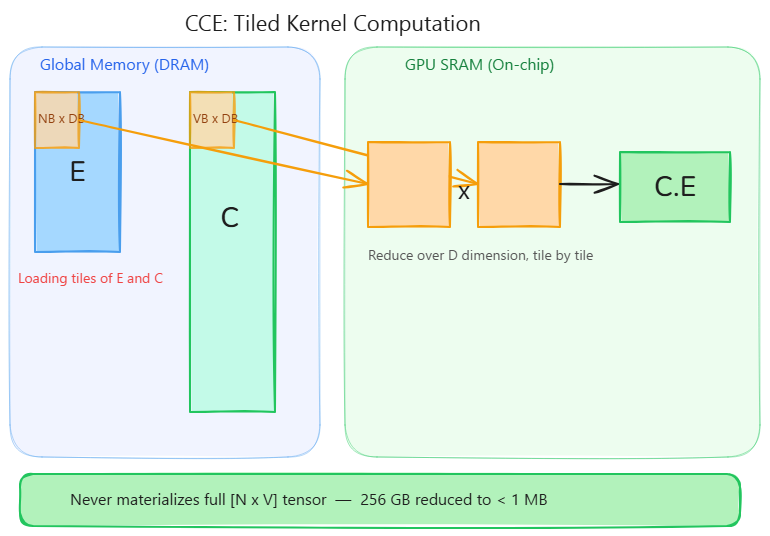
\[ 8*80000*256128*2 = 256gb \]

about 256gb of memory, spent just computing the cross entropy loss, accounting for over 90% of the total memory use in training.

Cut Cross Entropy

Cut Cross Entropy paper approaches this problem by implementing efficient forward and backward passes using custom fused triton kernels, implementing ideas like tiling and indexed loads, together with the reformulation above. This approach ensures that only small chunks of E and C are loaded into the fast GPU shared memory, and by parallelizing across thread blocks, we don’t incure any meaningful latency overheads. The key idea is that if we never compute all V logits at once, we never need the large $ B, S, V $ tensors that takes so much memory in the first place.

Forward Pass Kernels

Since we already reformulated the cross entropy loss as:

\[ \ell_i(x) = - C^\top_{x_i} E_i + \log \sum_j \exp(C^\top_j E_i) \]

The cut cross entropy paper breaks the terms above into two separate triton kernels in the forward pass:

An indexed Negative Dot Product
The Log Sum Exp

Indexed Negative Dot Product

A naive computation of the indexed matrix multiplication involves either indexing the classifier weight matrix ($C^\top$) with a memory cost of $ O(ND) $ , and then performing the dot product, or computing $\left(C^\top_{x_i} E_i\right)$ which materializes the logits for every token and then indexing into the result to get the logit for the target class, with an $O(N|V|)$ memory cost.

Cut Cross Entropy uses a tiled approach,

Indexed Matrix Multiplication

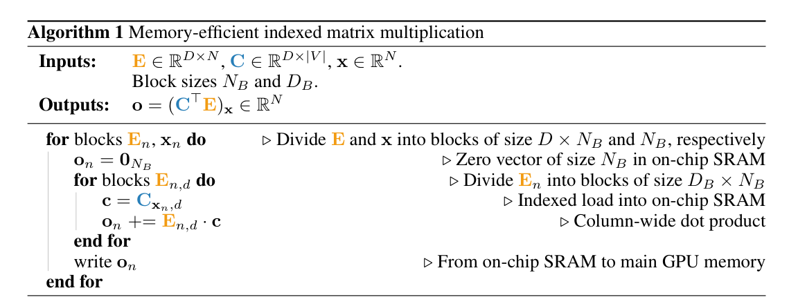
Each thread block computes $N_B$ dot products for $N_B$ tokens from the input sequence and writes them to O in global memory.
For a token position $i$ in an input sequence, to compute $\left(C^\top E_i\right)$, we only load $x_i$ (the actual token value), $E_i$ and $C_{x_i}$ into the shared memory (SRAM) of our threadgroup.
Since we have limited shared memory, we can’t load the full hidden states $E(N_B, D)$ and $C(N_B, D)$, that we need to calculate the dot product for the $N_B$ tokens.
We break $E$ and $C$ into tiles of size $(N_B, D_B)$ and $(N_B, D_B)$ respectively, and compute the dot product for these tiles, iterating over the D (reduction) dimension of E and C and accumulating the dot product in GPU shared memory, before writing to O in global memory. Here’s my naive implementation:

def indexed_dot_kernel(
    E_ptr,  # Hidden states 
    C_ptr,  # Model's Classifier weight matrix
    x_ptr,  # target tokens
    O_ptr,  # where are we writing dot products to?
    N,  # sequence_length
    D,  # Hidden_Dim
    V,  # Vocab size
    BLOCK_N: tl.constexpr,  # Block size across x, how many tokens is this block attending to
    BLOCK_D: tl.constexpr,  # how much of E are we loading at once across the D dimension
    stride_en,
    stride_ed,
    stride_cv,
    stride_cd,
):
    pid = tl.program_id(axis=0)  # what tokens am I handling in the input sequence?

    x_offsets = pid * BLOCK_N + tl.arange(0, BLOCK_N)  # computing address offsets
    x_mask = x_offsets < N

    # loading target token indices

    x = tl.load(x_ptr + x_offsets, mask=x_mask, other=0) 
    # temporary tensor to store dot products for NB tokens in SRAM
    o = tl.zeros([BLOCK_N], dtype=tl.float32)
    # reduction over D
    for d in range(0, D, BLOCK_D):
        d_offsets = d + tl.arange(0, BLOCK_D)
        # loading E tile
        e = tl.load(
            E_ptr + x_offsets[:, None] * stride_en + d_offsets[None, :] * stride_ed,
            mask=(x_offsets[:, None] < N) & (d_offsets[None, :] < D),
            other=0.0
        )
        # loading C tile
        c = tl.load(
            C_ptr + x[:, None]*stride_cv + d_offsets[None, :] * stride_cd,
            mask=(x[:,None] < V) & (d_offsets[None, :] < D),
            other=0.0
        )
        # accumulating
        o += tl.sum((e*c).to(tl.float32), axis=1)
    # writing back to global memory
    tl.store(O_ptr + x_offsets, -o, mask=x_mask)

Each threadblock loads NB tokens, performs reduction over the D dimensions of the hidden states, and loads up tiles of $E$ and $C$, performs the dot product and accumulates the result over each tile. However, this is not efficient enough as we only parallelize of the token sequence length N, and would end up utilizing less than 60% of our Streaming Multiprocessors as D gets larger. Since we only launch $N / N_B$ threadblocks, if we had N = 2048, D = 4096, $N_B$ = 64, and BLOCK_D = 256, on an A100 with 108 Streaming Multiprocessors, our kernel launches only 32 programs (cdiv(2048, 64)), utilizing less than 30% of the GPU.

The official apple implementation however, parellizes over both tokens and hidden dimensions, using a 2D logical kernel grid, that saturates the GPUs Streaming Multiprocessors with enough work.

    def _indexed_neg_dot_forward_kernel(
        E,
        C,
        Inds,
        Valids,
        Out,
        B,
        D,
        stride_eb,
        stride_ed,
        stride_cv,
        stride_cd,
        stride_ib,
        stride_vb,
        B_BIN,
        BLOCK_B: tl.constexpr,
        BLOCK_D: tl.constexpr,
        GROUP_B: tl.constexpr,
        HAS_VALIDS: tl.constexpr,
        EVEN_D: tl.constexpr,
        SHIFT: tl.constexpr,
    ):
        pid = tl.program_id(axis=0)
        num_b_chunks = tl.cdiv(B, BLOCK_B)
        num_d_chunks = tl.cdiv(D, BLOCK_D)
        num_d_in_group = GROUP_B * num_d_chunks
        group_id = pid // num_d_in_group
        first_pid_b = group_id * GROUP_B
        group_size_b = min(num_b_chunks - first_pid_b, GROUP_B)
        pid_b = first_pid_b + ((pid % num_d_in_group) % group_size_b)
        pid_d = (pid % num_d_in_group) // group_size_b

        offs_b = (tl.arange(0, BLOCK_B) + pid_b * BLOCK_B) % B
        if HAS_VALIDS:
            offs_b = tl.load(Valids + stride_vb * offs_b)

        offs_d = tl.arange(0, BLOCK_D) + pid_d * BLOCK_D
        e_ptrs = E + (stride_eb * offs_b[:, None] + stride_ed * offs_d[None, :])
        if EVEN_D:
            e = tl.load(e_ptrs)
        else:
            e = tl.load(e_ptrs, mask=offs_d[None, :] < D, other=0.0)

        inds = tl.load(Inds + stride_ib * ((offs_b + 1) if SHIFT else offs_b))

        c_ptrs = C + (inds[:, None] * stride_cv + offs_d[None, :] * stride_cd)
        if EVEN_D:
            c = tl.load(c_ptrs)
        else:
            c = tl.load(c_ptrs, mask=offs_d[None, :] < D, other=0.0)

        offs_b = tl.arange(0, BLOCK_B) + pid_b * BLOCK_B
        out_ptrs = Out + offs_b
        dot = (e * c).to(tl.float32)
        neg_dot = -tl.sum(dot, 1).to(out_ptrs.dtype.element_ty)
        tl.atomic_add(out_ptrs, neg_dot, mask=offs_b < B)

This way multiple thread blocks can compute over the same $E$ tile, which introduces a need to synchronize the multiple threads writing to the same address in O(minimal overhead compared to the cost of underutilizing the gpu), this synchronization is done by :

tl.atomic_add(out_ptrs, neg_dot, mask=offs_b < B)

Log-Sum-Exp

The second part of our equation, the Log-Sum-Exp, is also implemented using a similar approach Efficient Log-Sum-Exp

Again:

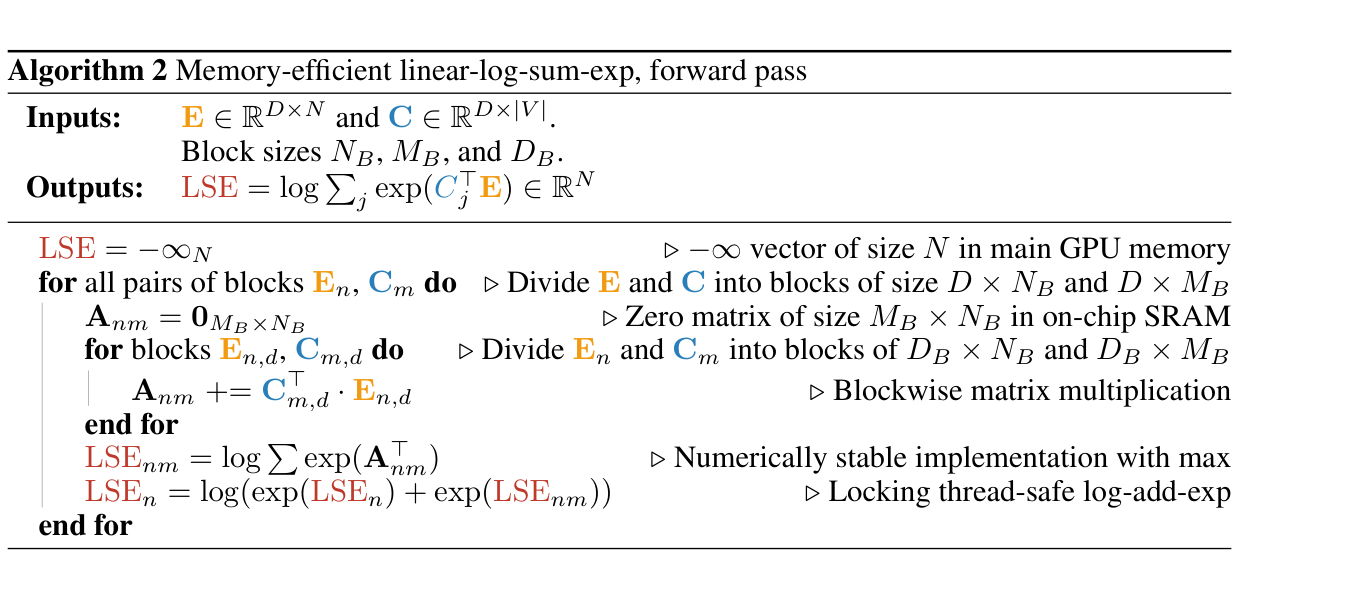
Each threadblock computes the partial log sum exp for $N_B$ tokens
We parallelize over both NB(tokens) and VB (vocab size), to avoid loading up the full C matrix into SRAM for each token.

def _cce_lse_forward_kernel(
    E,
    C,
    LSE,
    LA,
    Locks,
    Valids,
    softcap,
    B,
    V,
    D,
    stride_eb,
    stride_ed,
    stride_cv,
    stride_cd,
    stride_lse_b,
    stride_vb,
    num_locks,
    # Meta-parameters
    B_BIN,
    HAS_VALIDS: tl.constexpr,
    BLOCK_B: tl.constexpr,
    BLOCK_V: tl.constexpr,
    BLOCK_D: tl.constexpr,  #
    GROUP_B: tl.constexpr,  #
    EVEN_D: tl.constexpr,
    HAS_SOFTCAP: tl.constexpr,
    HAS_LA: tl.constexpr,
    DOT_PRECISION: tl.constexpr,
):
    pid = tl.program_id(axis=0)
    num_pid_b = tl.cdiv(B, BLOCK_B)
    num_pid_v = tl.cdiv(V, BLOCK_V)
    num_pid_in_group = GROUP_B * num_pid_v
    group_id = pid // num_pid_in_group
    first_pid_b = group_id * GROUP_B
    group_size_b = min(num_pid_b - first_pid_b, GROUP_B)
    pid_b = first_pid_b + ((pid % num_pid_in_group) % group_size_b)
    pid_v = (pid % num_pid_in_group) // group_size_b

    offs_b = (pid_b * BLOCK_B + tl.arange(0, BLOCK_B)) % B
    if HAS_VALIDS:
        offs_b = tl.load(Valids + stride_vb * offs_b)

    offs_v = (pid_v * BLOCK_V + tl.arange(0, BLOCK_V)) % V
    offs_d = tl.arange(0, BLOCK_D)
    e_ptrs = E + (offs_b[:, None] * stride_eb + offs_d[None, :] * stride_ed)
    c_ptrs = C + (offs_v[None, :] * stride_cv + offs_d[:, None] * stride_cd)

We use reduction to avoid loading up either E or C across the entire D Dimension, so we only ever load $E(N_B, D_B)$ and $C(V_B, D_B)$ at any point in time, accumulating the dot products in $\text{accum}$ in shared memory. $\text{accum}$ now contains partial logits for the $N_B$ tokens, since it was computed from $E(N_B, D)$ and $C(D, V_B)$, and not the full $C(D, V)$

tiled_matmul

    accum = tl.zeros((BLOCK_B, BLOCK_V), dtype=tl.float32)
    for d in range(0, tl.cdiv(D, BLOCK_D)):
        # Load the next block of E and C, generate a mask by checking the K dimension.
        # If it is out of bounds, set it to 0.
        if EVEN_D:
            e = tl.load(e_ptrs)
            c = tl.load(c_ptrs)
        else:
            e = tl.load(e_ptrs, mask=offs_d[None, :] < D - d * BLOCK_D, other=0.0)
            c = tl.load(c_ptrs, mask=offs_d[:, None] < D - d * BLOCK_D, other=0.0)
        accum = tl.dot(e, c, accum, input_precision=DOT_PRECISION)
        e_ptrs += BLOCK_D * stride_ed
        c_ptrs += BLOCK_D * stride_cd

The log sum exp over the partial logits is now computed by finding the max of the logits over this $V_B$ block, substracting it from all logits, calculate the exponent, the sum of the exponents over the $V$ axis, and finally the log of the sums. This value is stored in this_lse in shared memory.

    this_mx = tl.max(logits, axis=1)
    e = tl.exp(logits - this_mx[:, None])
    this_lse = this_mx + tl.log(tl.sum(e, axis=1))

Remember, we only have computed partial logits of size $(N_B, V_B)$ at this point, since each thread block computes the logits over a $V_B$ portion of the model’s vocabulary. $\text{this\_lse}$ holds the log-sum-exp for the partial logits of a particular thread block, which is not the full value we need. However, at this point, other threadblocks with the same $\text{pid\_b}$ (handling the same token block), and different values for $\text{pid\_v}$ (handling different blocks of $V$), would have also calculated their $\text{this\_lse}$ values for the other $(V_B)$ blocks in V, we need to find a way to sum these values without introducing race conditions across these threadblocks.

    lse_ptrs = LSE + (stride_lse_b * off_b)

    this_locks = Locks + (pid_b // tl.cdiv(B, BLOCK_B * num_locks))
    while tl.atomic_cas(this_locks, 0, 1) == 1:
        pass
    lse = tl.load(lse_ptrs, mask=o_mask, other=0.0, eviction_policy="evict_last")
    lse = tl_logaddexp(lse, this_lse)
    tl.store(lse_ptrs, lse, mask=o_mask, eviction_policy="evict_last")

    tl.atomic_xchg(this_locks, 0)

The final log-sum-exp are stored at $\text{LSE}$, however since multiple thread blocks with the same $\text{pid\_b}$ will write to the same address in $\text{LSE}$, a spin atomic lock is used to prevent race conditions, and the current program holding the lock loads the current value for $\text{LSE}$ into $\text{lse}$ in it’s shared memory, and adds it to it’s partial logits computed in this_lse with the logaddexp function, and writes the new computed $\text{LSE}$ value back to LSE in global memory before releasing the lock for other threadblocks. The full log sum exp is the final value in LSE when all threadblocks have released the lock. We can add multiple partial log-sum-exps in this manner because : \[ log(\exp(a) + \exp(b)) = a + \log(1 + \exp(b-a)) \] which is basically what the tl_logaddexp function does.

Together, these two kernels compute the full cross entropy loss without ever materializing a tensor larger than $[N_B, V_B]$ in memory, drastically reducing GPU global memory consumption, and effectively utilizing the GPU’s streaming multiprocessors.

Backward Pass

The backward pass for cross entropy produces two gradients, ∂L/∂E and ∂L/∂C, however computing these gradients naively also requires large intermediate tensors that cannot fit in GPU memory. In this section, we look at how the gradients are reformulated before diving into the backward pass kernels.

Since the cross entropy loss is given as :

\[ \ell_i(x) = - C^\top_{x_i} E_i + \log \sum_j \exp(C^\top_j E_i) \]

The computation graph of the forward pass through the model can be summarized in the image below:

computation graph

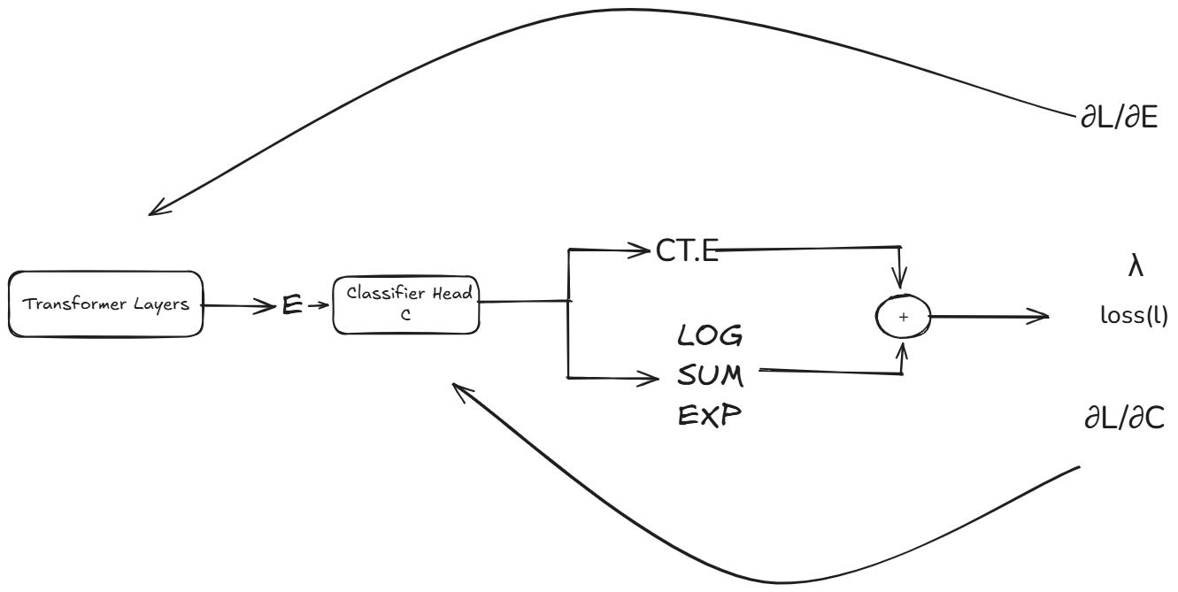
At the cross entropy loss calculation node on the graph, we need to compute local gradients ∂L/∂E and ∂L/∂C, why? because for every operation on the autograd computation graph, we must compute a local gradient with respect to it’s inputs, using the formula :

node_gradient = local_gradient x grad_out

grad_out = gradient from the next node in the graph (backpropagating back to this node)

For the cross entropy loss, the models’s hidden states $E$ and classifier weight matrix $C$ were the inputs, thus our required gradients are ∂L/∂E and ∂L/∂C.

∂L/∂E backpropagates back into the transformer layers and is backpropagated to compute other gradients down the graph, while ∂L/∂C into the classifer head and is used to compute the updates to the model’s classifer weights at each step.

As we can see, the CCE node branches into two nodes $\left(C^\top_{x_i} E_i\right)$ and $\log \sum_j \exp(C^\top_j E_i)$, thus our gradients ∂L/∂E and ∂L/∂C, are made of two parts, one from the indexed-dot product $\left(C^\top_{x_i} E_i\right)$, and the other from the log-sum-exp $\log \sum_j \exp(C^\top_j E_i)$.

The key intuition behind both gradients is that they reduce to the difference between the model’s softmax predictions and the ground truth one-hot label $\mathbf{1}_{x_i}$ (the target tokens). For every other token $j \neq x_i$ in the vocabulary, the gradient is simply the softmax value itself. This difference, softmax minus one-hot, is what drives the model’s weights toward assigning higher probability to the correct token at each training step.

Let’s look at how the first gradient ∂L/∂E is calculated

\[ \frac{\partial \ell_i}{\partial E_i} = -C_{x_i} + \frac{\partial}{\partial E_i} \log \sum_j \exp(C^\top_j E_i) \]

Next, we expand the log-sum-exp derivative using the chain rule

\[ \frac{\partial}{\partial E_i} \log \sum_j \exp(C^\top_j E_i) = \frac{\sum_j C_j \exp(C^\top_j E_i)}{\sum_j \exp(C^\top_j E_i)} = \sum_j C_j \cdot \text{softmax}_j(C^\top E_i) \]

which gives ∂L/∂E as

\[ \frac{\partial \ell_i}{\partial E_i} = -C_{x_i} + \sum_j C_j \cdot S_{i,j} \]

where $S_{i,j}$ = $\text{softmax}_j(C^\top E_i)$

This is expressed in compact matrix form as:

\[ \nabla E_i = \sum_j C_j \cdot S_{i,j} - C_{x_i} \]

∂L/∂C follows a similar pattern, but we now differentiate with respect to the classifier weight $C_j$:

\[ \nabla C_j = -E_i \,\mathbf{1}_{j = x_i} + \frac{\partial}{\partial C_j} \log \sum_k \exp(C^\top_k E_i) \]

the derivative of the log-sum-exp with respect to $C_j$ is:

\[ \frac{\partial}{\partial C_j} \log \sum_k \exp(C^\top_k E_i) = S_{i,j} \cdot E_i \]

thus:

\[ \nabla C_j = (S_{i,j} - \mathbf{1}_{j = x_i}) \cdot E_i \]

and in compact matrix form:

\[ \nabla C = \hat{S}^\top E \]

Both gradients, ∂L/∂C and ∂L/∂E require two matrix multiplications, $(C^\top_j E_i)$ with size $[N,V]$ and $\hat{S}C$ or $\hat{S}^\top E$. and the intermediate matrix $\hat{S}$ of size $[N,V]$ that doesn’t fit into GPU memory, we also perform non-linear operations on these tensors to calculate the softmax.

Before we go into the kernels, we also note that $\nabla C$ has shape $[V,D]$ and $\nabla E$ has shape $[N,D]$, the same as $\text{C}$ and $\text{E}$ respectively

CCE backward pass kernel

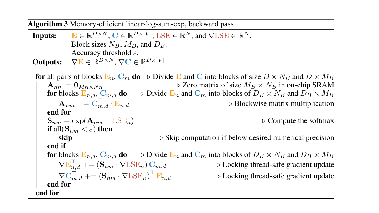
The backward kernel above computes $\nabla C$ and $\nabla E$ in one kernel. It reuses the same tiling approach from the log-sum-exp kernel to compute the matrix multiplication $\left(C^\top_{x_i} E_i\right)$. We reuse the $\text{LSE}$ value computed in the forward pass to calculate the softmax since

\[ S_{i,j} = \frac{\exp(C^\top_j E_i)}{\sum_k \exp(C^\top_k E_i)} \]

Since $\text{LSE}_i = \log \sum_k \exp(C^\top_k E_i)$, the denominator of the softmax is simply $\exp(\text{LSE}_i)$:

\[ S_{i,j} = \frac{\exp(C^\top_j E_i)}{\exp(\text{LSE}_i)} = \exp(C^\top_j E_i - \text{LSE}_i) \]

So the compact connection is:

\[ S = \exp(C^\top E - \text{LSE}) \]

Finally, we can go through the kernel

The backward kernel calculates the addresses for $E$ and $C$ exactly the same as the LSE kernel we previously looked at.

def _cce_backward_kernel(
    E,
    C,
    LSE,
    dOut,
    grad_scale,
    Valids,
    VocabOrdering,
    softcap,
    Targets,
    dE,
    dELocks,
    dC,
    dCLocks,
    B,
    D,
    V,
    n_de_locks_0,
    n_de_locks_1,
    n_dc_locks_0,
    n_dc_locks_1,
    stride_eb,
    stride_ed,
    stride_cv,
    stride_cd,
    stride_vb,
    filter_eps,
    B_BIN,
    BLOCK_B: tl.constexpr,
    BLOCK_V: tl.constexpr,
    BLOCK_D: tl.constexpr,
    MM_BACK_BLOCK_D: tl.constexpr,
    GROUP_B: tl.constexpr,
    EVEN_D: tl.constexpr,
    MM_BACK_EVEN_D: tl.constexpr,
    ITEM_DO: tl.constexpr,
    HAS_VALIDS: tl.constexpr,
    HAS_VOCAB_ORDERING: tl.constexpr,
    FILTER_GRAD: tl.constexpr,
    HAS_TARGETS: tl.constexpr,
    HAS_SOFTCAP: tl.constexpr,
    SHIFT: tl.constexpr,
):
    pid = tl.program_id(axis=0)
    num_b_chunks = tl.cdiv(B, BLOCK_B)
    num_v_chunks = tl.cdiv(V, BLOCK_V)
    num_v_in_group = GROUP_B * num_v_chunks
    group_id = pid // num_v_in_group
    first_pid_b = group_id * GROUP_B
    group_size_b = min(num_b_chunks - first_pid_b, GROUP_B)
    pid_b = first_pid_b + ((pid % num_v_in_group) % group_size_b)
    pid_v = (pid % num_v_in_group) // group_size_b

    offs_b = (pid_b * BLOCK_B + tl.arange(0, BLOCK_B)) % B
    if HAS_VALIDS:
        offs_b = tl.load(Valids + stride_vb * offs_b)

    offs_v = (pid_v * BLOCK_V + tl.arange(0, BLOCK_V)) % V
    if HAS_VOCAB_ORDERING:
        offs_v = tl.load(VocabOrdering + offs_v)

    offs_d = tl.arange(0, BLOCK_D)
    e_ptrs = E + (offs_b[:, None] * stride_eb + offs_d[None, :] * stride_ed)
    c_ptrs = C + (offs_v[None, :] * stride_cv + offs_d[:, None] * stride_cd)

we calculate $(C^\top_j E_i)$ exactly the same way as we did in the LSE kernel, computing partial Logits $[NB, VB]$, utilizing reduction over the D dimension and accumulating the dot products in accum

    for d in range(0, tl.cdiv(D, BLOCK_D)):
        if EVEN_D:
            e = tl.load(e_ptrs)
            c = tl.load(c_ptrs)
        else:
            e = tl.load(e_ptrs, mask=offs_d[None, :] < D - d * BLOCK_D, other=0.0)
            c = tl.load(c_ptrs, mask=offs_d[:, None] < D - d * BLOCK_D, other=0.0)

        accum = tl.dot(e, c, accum)

        e_ptrs += BLOCK_D * stride_ed
        c_ptrs += BLOCK_D * stride_cd

we load our LSE values from the forward pass, and calculate the softmax on the partial logits using \[S = \exp(C^\top E - \text{LSE})\]. The softmax is stored in d_accum

if HAS_VALIDS:
        lse = tl.load(LSE + (pid_b * BLOCK_B + tl.arange(0, BLOCK_B)) % B)
    else:
        lse = tl.load(LSE + offs_b)

    d_accum = tl.exp(accum - lse[:, None])

At this point d_accum holds $\text{softmax}_j(C^\top E_i)$ for the current $[N_B, V_B]$ tile. We now apply the one-hot subtraction from our gradient derivation. Recall that $\partial \ell / \partial C$ has two parts: a positive contribution from the log-sum-exp term, and a negative contribution from the indexed dot product term $-C^\top_{x_i} E_i$. Differentiating that second term with respect to $C_j$ gives $-E_i$ when $j = x_i$ and $0$ everywhere else — exactly the $-\mathbf{1}_{j=x_i}$ in $\nabla C_j = (S_{i,j} - \mathbf{1}_{j=x_i}) \cdot E_i$. is_target is a boolean matrix of shape $[N_B, V_B]$, True wherever $j = x_i$, and tl.where uses it to add $-1.0$ at those positions. After this step, d_accum holds $\text{softmax}_j(C^\top E_i) - \mathbf{1}_{j = x_i}$, which is exactly $\hat{S}$ from our gradient formula.

    if HAS_TARGETS:
        targets = tl.load(Targets + ((offs_b + 1) if SHIFT else offs_b))
        is_target = targets[:, None] == offs_v[None, :]
        d_accum += tl.where(is_target, -1.0, 0.0)

At this point, d_accum holds the softmax over NB tokens the program is holding, and has a shape $[NB, VB]$. The next thing to do is to compute the matrix multiplication of $\text{softmax}_j(C^\top E_i)$ for ∂L/∂E and softmax $\text{softmax}_j(C^\top E_i)$ and $E$ for ∂L/∂C.

We write a simple matmul kernel to avoid rewriting the same code twice, passing arguments softmax(ct.E), E or C where neccessary

@triton.jit
def _mm_backward(
    do,
    da_ptrs,
    partial_mask_a,
    da_lock_ptr,
    n_locks,
    b_ptrs,
    partial_mask_b,
    stride_ad,
    stride_bd,
    D,
    BLOCK_D: tl.constexpr,
    EVEN_D: tl.constexpr,
):
    d_inds = tl.arange(0, BLOCK_D)[None, :]

    da_ptrs = da_ptrs + d_inds * stride_ad
    b_ptrs = b_ptrs + d_inds * stride_bd

    for d in range(0, tl.cdiv(D, BLOCK_D)):
        if EVEN_D:
            mask = partial_mask_b
        else:
            mask = partial_mask_b & (d_inds < (D - d * BLOCK_D))

        b = tl.load(b_ptrs, mask=mask, other=0.0)

        da_i = tl.dot(do, b).to(da_ptrs.dtype.element_ty)

        if EVEN_D:
            mask = partial_mask_a
        else:
            mask = partial_mask_a & (d_inds < (D - d * BLOCK_D))

        lock_offset = d // tl.cdiv(D, BLOCK_D * n_locks)
        this_da_lock_ptr = da_lock_ptr + lock_offset

        tl_lock_add(da_ptrs, da_i, mask, this_da_lock_ptr)

        b_ptrs += BLOCK_D * stride_bd
        da_ptrs += BLOCK_D * stride_ad

Looking at the above kernel carefully, our backward kernel computes $\hat{S} = \text{softmax}(C^\top E) - \mathbf{1}_{j=x_i}$ over $[N_B, V_B]$ tiles, because we don’t want to materialize the full $\hat{S}\ [N, V]$ in memory. When calculating $\partial \ell / \partial C$, the tile $\hat{S}\ [N_B, V_B]$ multiplied by $C\ [V_B, D]$ produces $[N_B, D]$ as expected, but these are only partial values of $\partial \ell / \partial C$. The actual matrix multiplication is over $\hat{S}\ [N, V]$ (the entire vocab) and $C\ [V, D]$. Our tiled approach works because we parallelized over both $N$ and $V$ when launching the kernel. Just like the LSE kernel, multiple thread blocks share the same $\text{pid\_b}$ (operating over the same $N_B$ tokens) but hold different $\text{pid\_v}$ values, each computing their portion of $V$. We use a lock to accumulate contributions from all thread blocks covering the same $N_B$ tokens, so the final gradient value matches what we would have obtained by multiplying the full $\hat{S} \cdot C$ in global memory.

Computing ∂L/∂C is straightforward, we pass args, d_accum (softmax), pointers to read E$[NB, D]$ and write to ∂L/∂C, locks, and other params we need for the tiled matmul.

   _mm_backward(
        tl.trans(d_accum),
        dC + (offs_v[:, None] * stride_cv),
        v_mask,
        dCLocks,
        n_dc_locks_1,
        E + (offs_b[:, None] * stride_eb),
        b_mask,
        stride_cd,
        stride_ed,
        D,
        MM_BACK_BLOCK_D,
        MM_BACK_EVEN_D,
    )

The same applies to ∂L/∂E, we again pass the pointers to the softmax S, $C$

  _mm_backward(
        d_accum,
        dE + (offs_b[:, None] * stride_eb),
        b_mask,
        dELocks,
        n_de_locks_1,
        C + offs_v[:, None] * stride_cv,
        v_mask,
        stride_ed,
        stride_cd,
        D,
        MM_BACK_BLOCK_D,
        MM_BACK_EVEN_D,
    )

The backward pass kernel takes slightly more memory than the forward pass, since we compute two matrix multiplications in one kernel.

We have now seen how we compute the gradients of the cross entropy loss function without ever materializing a tensor large than $[NB, VB]$ in memory.

Benchmarking Gemma4

Finally, I benchmarked cut cross entropy against torch_compile and vanilla cross entropy in two ways:

I ran a script that runs local inference through gemma4-2b-instruction_tuned on the alpaca dataset that generetes hidden states $E$, target labels $x$, and extracts $C$, the classifier head of gemma4, and then uses CCE, toch_compile, and vanilla cross entropy to calculate the loss and gradients on these inputs , measuring peak GPU memory usage before and after running the loss computations.

for this_test_data in tqdm.tqdm(
        test_data, desc="Data source", disable=len(test_data) == 1
    ):
        gen = data.generator(this_test_data)
        for rep in tqdm.trange(n_rep + 1, desc="Repetition"):
            D = gen(dtype=dtype)
            for kind in tqdm.tqdm(
                kinds, desc="Benchmark kind", disable=len(kinds) == 1
            ):
                E, C, T = D.embedding, D.classifier, D.targets

                this_softcap = softcap if softcap is not None else D.softcap

                kwargs: dict[str, Any] = {"softcap": this_softcap}
                if kind == "loss-fw":
                    E.requires_grad_(True)
                    C.requires_grad_(True)
                    args = (E, C, T)
                elif kind in {"loss-bw", "loss-fw-bw"}:
                    E.requires_grad_(True)
                    C.requires_grad_(True)

                    args = (E, C, T)
                    kwargs["backward"] = True
                    kwargs["forward"] = kind == "loss-fw-bw"
                    kwargs["pre_fn"] = clear_grad_fn
                else:
                    raise ValueError(f"Unknown kind {kind=}")

                for m in tqdm.tqdm(methods, desc="Method", leave=False):
                    if m in "liger" and kind.startswith("lse"):
                        continue
                    print(f"Loss calculated with {m}")

                    # warmup (it==0)
                    stats = memory.Stats.measure(
                        (
                            baseline
                            if m == "baseline"
                            else functools.partial(linear_cross_entropy, impl=m)
                        ),
                        *args,
                        n_iteration=n_iteration if rep > 0 else 1,
                        **kwargs,
                    )

This benchmark was done on a 40GB A100, with the results shown below :


============================================================
  gemma4  |  loss-fw-bw
============================================================
Method                  Time (ms)    Memory (MB)
-------------------- ------------ --------------
cce                         84.49          794.2
torch_compile               85.80         4888.0
baseline                   148.26        24576.0


============================================================
  mistral-nemo  |  loss-fw-bw
============================================================
Method                  Time (ms)    Memory (MB)
-------------------- ------------ --------------
torch_compile              130.71         3408.0
baseline                   154.69        12288.0
cce                        179.16         1361.4

Additionally I finetuned a base gemma4 (E-2b-it) on the full alpaca instruction tuning dataset, on an 80GB A100, with the full memory usage stats shown below